The Spread Alpha Atlas

The spread between two related assets is more predictable than either asset alone. I built 14 features on the Kalman-filtered residual of 15 pairs across futures, commodities, FX, equities, and crypto to find which ones carry tradeable signal.

Jul 23, 2026

∙ Paid

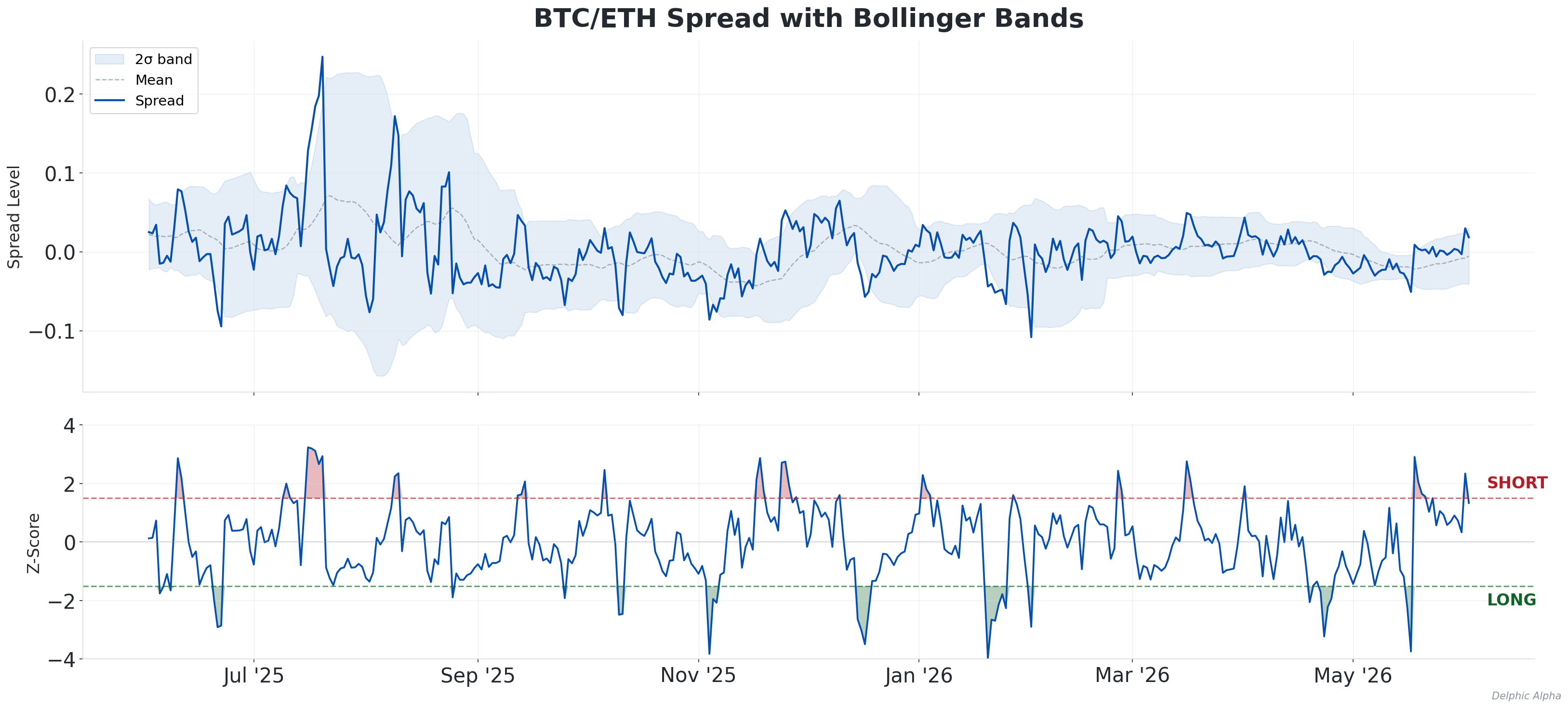
When two assets are structurally related (ES and NQ, gold and silver, BTC and ETH) their prices move together most of the time, but not all the time. The gap between them, the spread, captures these temporary divergences. Unlike individual prices, which trend and are hard to predict, spreads between related assets tend to be stationary and mean-reverting. That makes them a fundamentally different surface for alpha signals.

A spread alpha is a signal that predicts the direction of the spread's next move. If the BTC/ETH spread widens beyond its historical norm, a z-score signal flags the divergence and bets on reversion. If the signal is right more often than not, you have tradeable alpha on the spread.

But building spread alphas involves two decisions. First, how to construct the spread. Two assets rarely move dollar-for-dollar, so you need a hedge ratio that balances the contribution of each leg. Get it wrong and one leg dominates the spread, drowning out the signal. Second, which features to compute on that spread. Not all signals work, mean reversion thrives, momentum gets destroyed. I tested 14 feature families on 15 pairs across 5 asset classes and 3 timeframes to map which combinations produce tradeable alpha.

Dataset

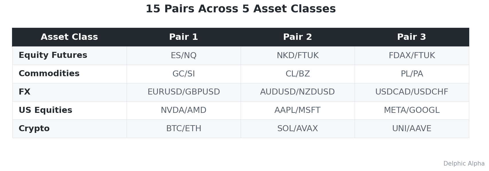
For each asset class I picked 3 representative pairs of structurally related assets, using data from January 2022 to July 2026.

Method

The Spread

The spread between two assets with prices P_base and P_quote is defined as:

where beta is the hedge ratio (how much of the base asset to hold against the quote) and c is an intercept that absorbs the average level difference. When beta = 1 and c = 0, this reduces to the simple log-ratio. But for most pairs, beta is not 1. ES/NQ has beta around 1.2, GC/SI around 1.0, NVDA/AMD around 0.8. If you use beta = 1 when the true value is 1.5, the spread is contaminated by the base leg's excess movement and the features measure noise instead of genuine divergence.

The Hedge Ratio

I estimate beta using a Kalman filter, which models:

with beta and intercept c as hidden states that update at each bar. The filter adapts the hedge ratio over time without overreacting to noise. To avoid continuous rebalancing, the Kalman beta is frozen at each rebalance boundary: weekly for daily data, daily for 30-minute data.

Features and Signals

I compute 14 feature families on the Kalman-adjusted spread: z-score, momentum, rate of change, distance from mean, Bollinger %B, skewness, kurtosis, variance ratio, OU half-life, RSI, MACD, cross-leg correlation, return differential, and relative volatility. Full definitions are in the appendix. Each feature is evaluated at lookbacks of 5, 10, 20, and 50 bars.

Each feature is converted to a directional signal: sign(feature_value). A position of +1 means long $1 of quote and short $beta of base. A position of -1 means the reverse.

P&L

PnL per bar is the actual hedged position return:

where beta is the frozen Kalman hedge ratio from the last rebalance. This is the return you would realise by holding the hedged position. Daily PnL is summed across bars and annualised via sqrt(252). No leverage, no compounding. Costs are applied as turnover times round-trip bps (2 bps for futures/FX, 10 bps for equities/crypto).

Results

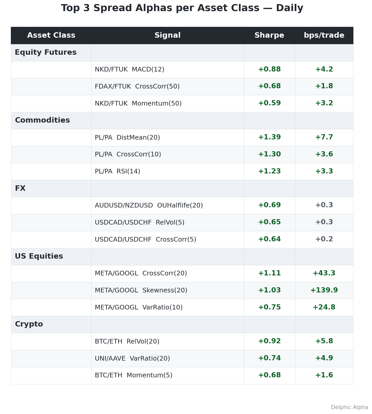
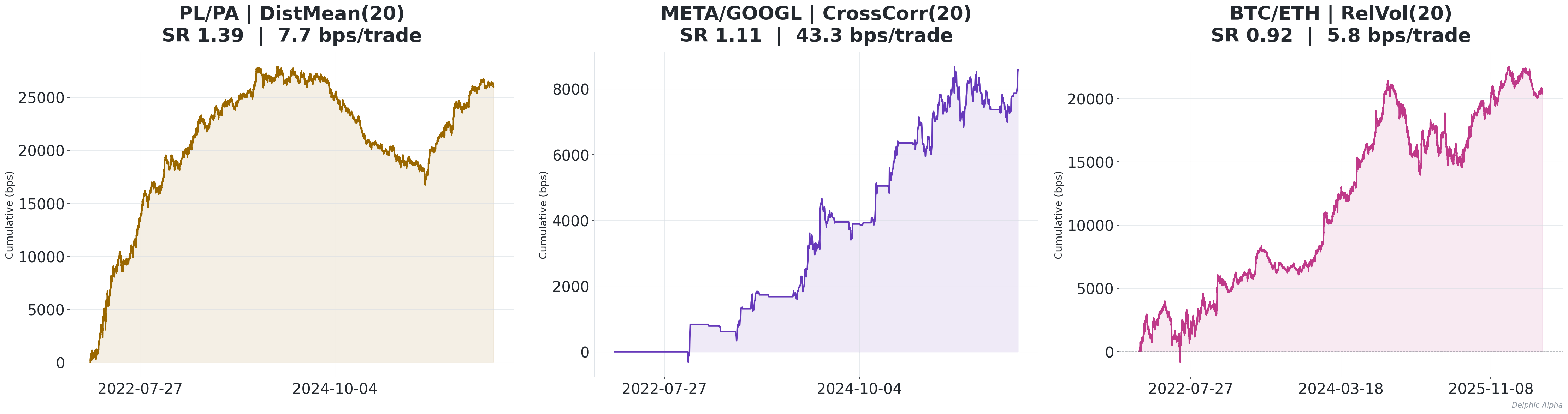
Daily: Top 3 per Asset Class

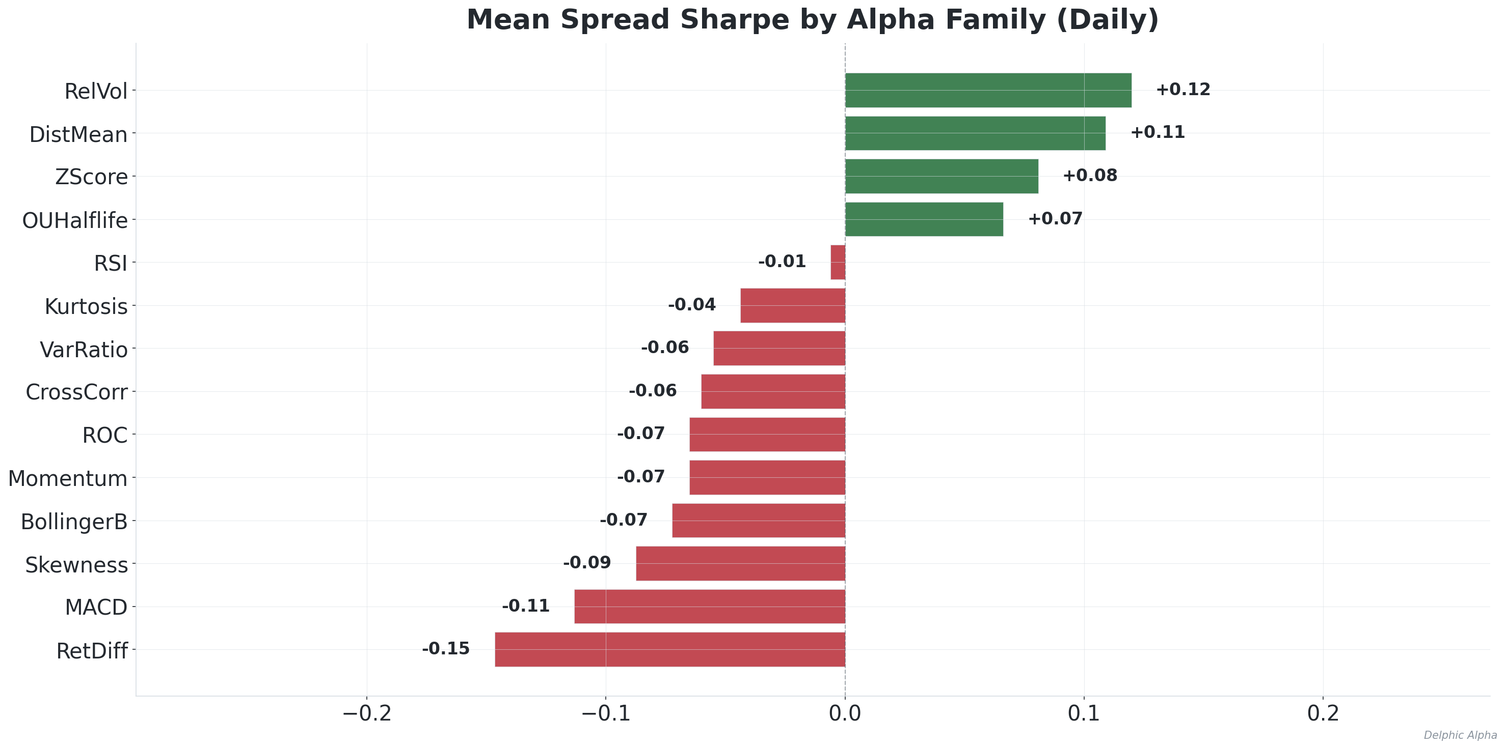
Sharpe by Alpha Family (Daily)

30-Minute: Top 3 per Asset Class

At 30-minute resolution the Kalman spread is rebalanced daily. The same feature families dominate but with higher Sharpe ratios due to more bars per day. These are gross figures. At intraday frequencies, execution costs will compress the net edge.

Delphic Alpha