Path Signatures: Does the Shape of Price Paths Predict Returns?

7 signals from rough path theory, 27 instruments, 4 asset classes, 4 timeframes. FadeVolRet: Sharpe +4.4, positive on all 8 crypto symbols for 5 consecutive years.

Every indicator you use on a rolling window, momentum, RSI, Bollinger bands, discards the order in which events occurred. Two 2-hour windows with identical total return and identical range expansion score identically, even if one saw price rally first and volatility respond, while the other saw volatility spike first and price catch up later. These are different market events (a breakout versus a news-driven gap) with different forward return profiles, but path-independent indicators cannot distinguish them.

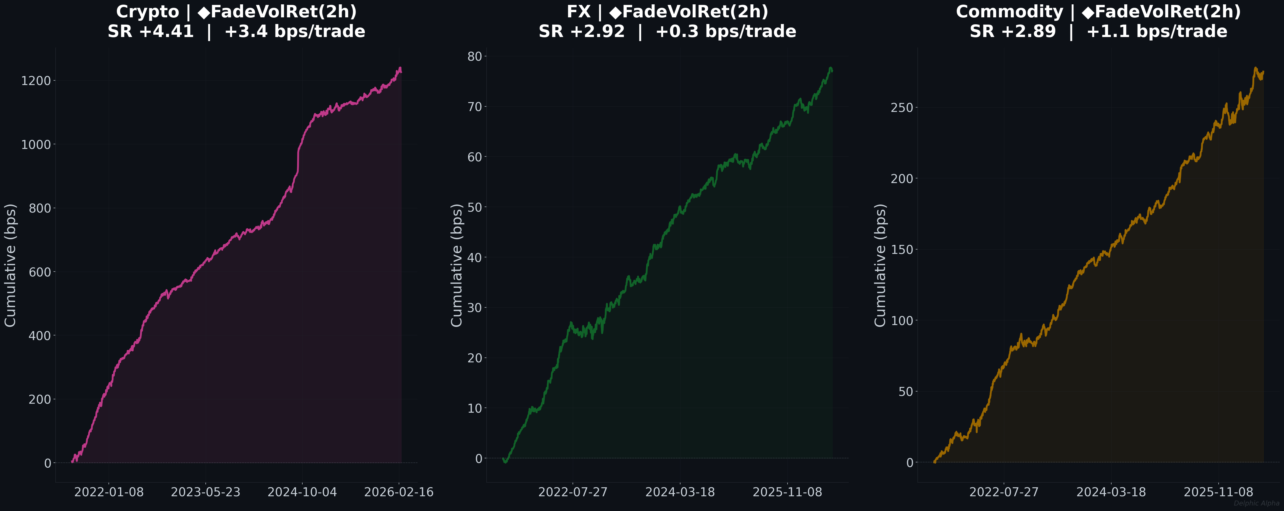
I tested whether this discarded ordering information contains tradeable alpha. Using path signatures from rough path theory, I built 7 signals that capture the shape of price paths and evaluated them across 27 instruments in 4 asset classes at 4 timeframes from daily to 5-minute bars. The strongest signal, FadeVolRet (fade the price move when volatility spikes first), produces Sharpe +4.4 in crypto at 5-minute frequency with +3.4 bps per trade. It is positive on all 8 crypto symbols individually and in 52 out of 56 months from 2021 to 2026.

Path signatures work by treating the rolling window not as a bag of bars but as a path: a curve traced through (return, volatility) space as time progresses. The signature decomposes this path into levels. Level 1 captures where price ended up, equivalent to simple momentum. Level 2 captures how it got there: acceleration, lead-lag between return and volatility, and the Levy area (the rotation between the two streams). These level 2 features encode the sequential structure that standard indicators throw away.

A practical property of signatures is that they are parameterisation-independent: they describe the geometry of the path regardless of sampling frequency. A 2% move over 5 minutes and a 2% move over 5 hours produce the same geometric description if the shape is the same. This makes them naturally robust to irregular sampling and time-of-day effects.

The Levy area is the most distinctive level 2 feature. It measures the signed area enclosed by the path in (return, volatility) space, capturing whether directional moves systematically precede or follow volatility expansion within the window. This separates momentum breakouts from mean-reverting vol spikes, a distinction no simple rolling statistic can make. Level 3 and above capture increasingly complex shape patterns, but level 2 is where the most interpretable features reside.

The question is whether these shape features produce alpha that simple momentum and volatility drift (level 1) do not. I constructed 7 signals: 2 controls from level 1, 5 shape signals from level 2. The evaluation covers 4 asset classes (equity futures, commodity futures, G7 FX, crypto), 4 timeframes (daily, hourly, 30-minute, 5-minute), and lookback windows from 5 days to 2 hours, totalling over 400 configurations tested on 5 years of data.

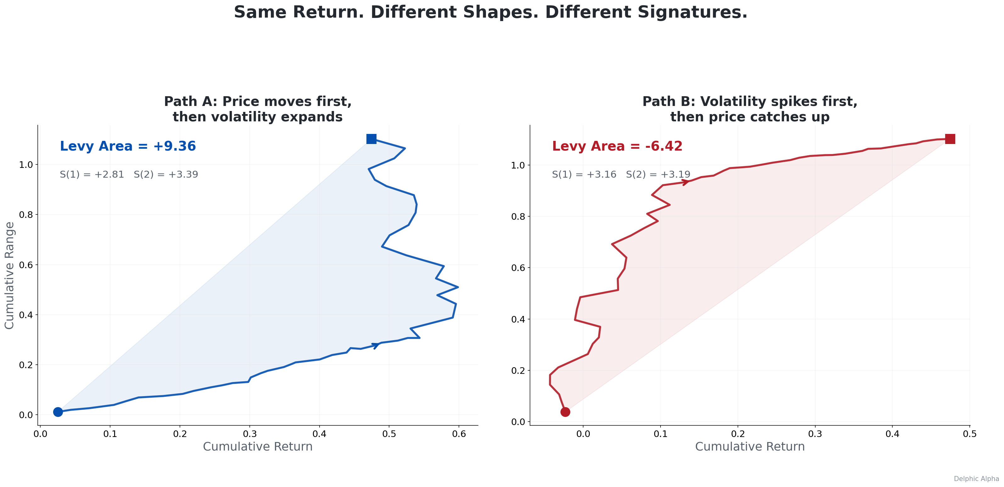
The illustration above demonstrates the core idea. Both paths end at the same return with the same total range. The level 1 signature components (S1, S2) are identical for both, as expected. However, the level 2 components diverge sharply. The Levy area, which measures the signed area enclosed by the path in (return, volatility) space, is +9.4 for the path where returns led volatility and -6.4 for the path where volatility led returns. The cross-terms S(1,2) and S(2,1) capture the same lead-lag structure from complementary angles. These level 2 features form the basis of the shape signals evaluated in this study.

Related: Simple Alpha Atlas (Daily) | Intraday Alpha Atlas (30M) | Spread Alpha Atlas

If you want to understand the broader alpha landscape that this study extends, the posts linked above test standard indicators (momentum, mean reversion, breakout, volatility) across the same asset classes and timeframes. The path signature signals evaluated here represent a new family of features that captures information those standard indicators discard.

Dataset

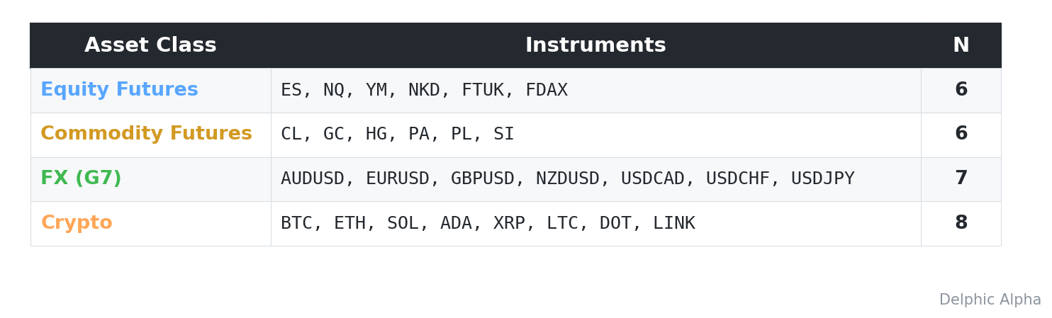
27 instruments from 4 asset classes, using data from July 2021 to July 2026.

Method

The Path

The first step is to construct a multi-dimensional path from the rolling window. At each bar within a window of length W, I record two quantities: the cumulative log return and the cumulative normalised range (high minus low, divided by close). Stacking these two streams produces a 2D path, a curve that traces how return and volatility evolved together over the window. The path is standardised to unit variance per dimension before computing the signature, which ensures that the resulting features are comparable across instruments and time periods with different volatility regimes.

Cumulative log return and cumulative normalised range, standardised to unit variance.

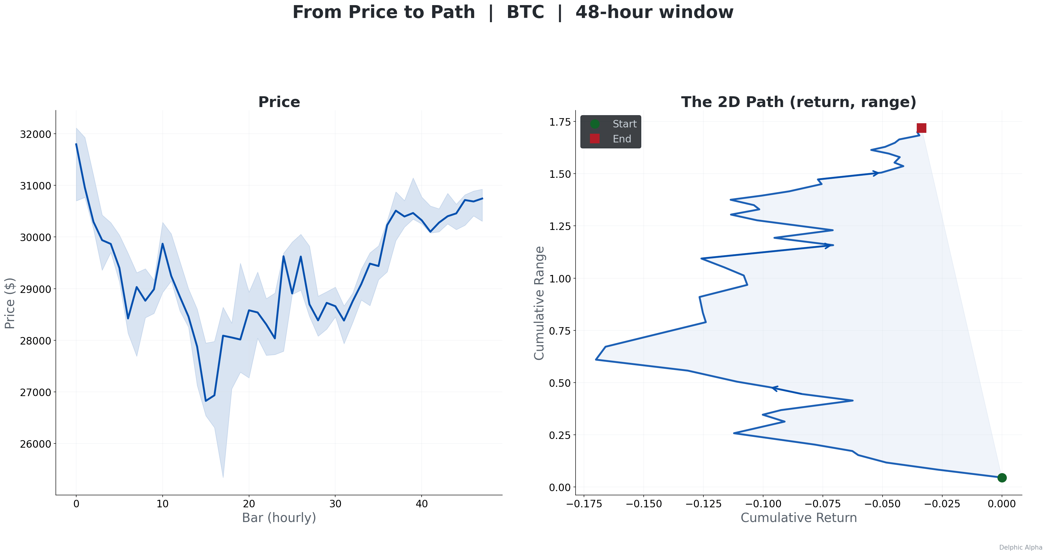
The figure above shows this construction on a 48-hour window of BTC price data. The raw OHLC data (left) is decomposed into per-bar log returns and normalised ranges (centre), which are then cumulatively summed to produce the 2D path (right). The shape of this path, its curvature, rotation, and the order in which the two streams evolve, is what the signature quantifies.

The choice of dimensions is important. Return and range are the two most fundamental properties of any price window, and their joint evolution over time captures the interaction between directional movement and volatility, the relationship that path-independent indicators reduce to a single summary statistic. A smooth uptrend with stable range traces a path that moves steadily along one axis. A volatility spike followed by a directional move traces a path that extends along the range axis first, then the return axis. These are geometrically distinct trajectories, and it is precisely this geometric distinction that the signature quantifies.

A natural extension is to add time as a third dimension (time augmentation), which would allow the signature to distinguish between paths that trace the same geometric shape at different speeds. One could also add order book imbalance, volume, or cross-asset returns as additional dimensions, each producing additional cross-terms at level 2 that capture lead-lag relationships between the new stream and the existing ones. In this study I restrict attention to the 2D (return, range) path to isolate the question of whether path shape alone carries alpha, before expanding to higher-dimensional paths in future work.

The Signature

The signature provides a systematic way to summarise the geometry of a path as a fixed-size vector. It is organised hierarchically. For a 2D path, the level 1 signature consists of two components: the total displacement in each dimension. For the (return, range) path, these are simply the total return and the total range change over the window, equivalent to standard momentum and volatility drift indicators. Level 1 is included as a control.

The level 2 signature consists of four additional components, each computed as a double sum over ordered pairs of increments within the path:

For each pair of dimensions i and j, sum the product of increment i at time t1 with increment j at time t2, over all ordered pairs t1 < t2.

No calculus is involved in the discrete case. On a time series of n bars, each level 2 component reduces to a sum over all pairs (i, j) where bar i precedes bar j. The four components have direct interpretations in the context of price dynamics:

S(1,1) = sum of return[i] * return[j] for all i < j. This captures return acceleration. When early returns are small and late returns are large (an accelerating move), S(1,1) takes a large positive value. When the reverse holds (a decelerating move), S(1,1) is smaller. Two windows with identical total return but different temporal profiles of that return produce different S(1,1) values.

S(1,2) = sum of return[i] * range_change[j] for all i < j. This captures return leading volatility. The component is large when directional price movements occur early in the window and range expansion follows, the characteristic pattern of a momentum breakout where the market reacts to a directional move with increased activity.

S(2,1) = sum of range_change[i] * return[j] for all i < j. This captures volatility leading return. The component is large when range expansion precedes directional price movement, the pattern observed before scheduled announcements or during liquidity-driven events where uncertainty manifests as widening ranges before price resolves in a direction.

S(2,2) = sum of range_change[i] * range_change[j] for all i < j. This captures volatility acceleration: whether the range is expanding at an increasing or decreasing rate over the window.

Of particular interest is the Levy area, defined as S(1,2) - S(2,1). This antisymmetric quantity measures the net difference between "return leads volatility" and "volatility leads return". Geometrically, it corresponds to the signed area enclosed by the path in (return, range) space. A positive Levy area indicates that the path rotates counterclockwise (returns precede volatility expansion). A negative Levy area indicates clockwise rotation (volatility expansion precedes returns). This feature has no equivalent among standard indicators, as it requires tracking the relative ordering of increments across two distinct streams simultaneously.

The iisignature Python library computes all six components (plus the derived Levy area) in microseconds per path via a recursive update formula known as the Chen identity, which avoids the naive O(n-squared) double loop over all pairs of bars.

Signals

Each of the 6 signature components (plus the derived Levy area) becomes a trading signal. Two are controls: Sig-Reversion = -S(1), a faded momentum signal equivalent to short-term mean reversion, and Sig-VolDrift = S(2), equivalent to range change. Five are shape signals: Sig-Accel = S(1,1), Sig-LevyArea = S(1,2) - S(2,1), Sig-FadeRetVol = -S(1,2), Sig-FadeVolRet = -S(2,1), and Sig-VolAccel = S(2,2). Three of these (Reversion, FadeRetVol, FadeVolRet) are negated because the raw signature components are consistently predictive of mean reversion: the natural trading direction is to fade the signal rather than follow it.

Each signal is z-scored over a 500-bar rolling window (how unusual is this path shape compared to recent history?), then discretised: long when z > 0, short when z < 0.

P&L

Position = sign(z-scored signal). PnL per bar:

z = rolling z-score of signature component, r = 1-bar forward return.

Equal-weight average across all symbols in each asset class. Daily PnL summed across bars and annualised via sqrt(252). No leverage, no compounding. bps/trade = total PnL in basis points divided by total position changes.

Results

Top Sharpe Signatures

The table below ranks the strongest signature configurations by |Sharpe| within each asset class (top 5 per class). Each row shows the signal family, timeframe, lookback, Sharpe ratio, bps per trade, and information coefficient (IC). The IC is the Spearman rank correlation between the z-scored signal and the subsequent 1-bar forward return, averaged across all symbols in the asset class.

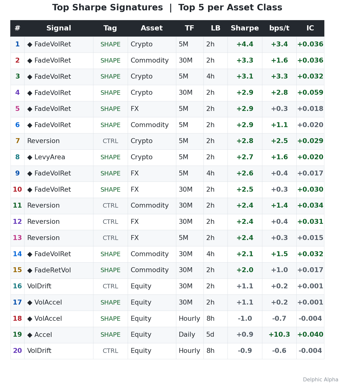
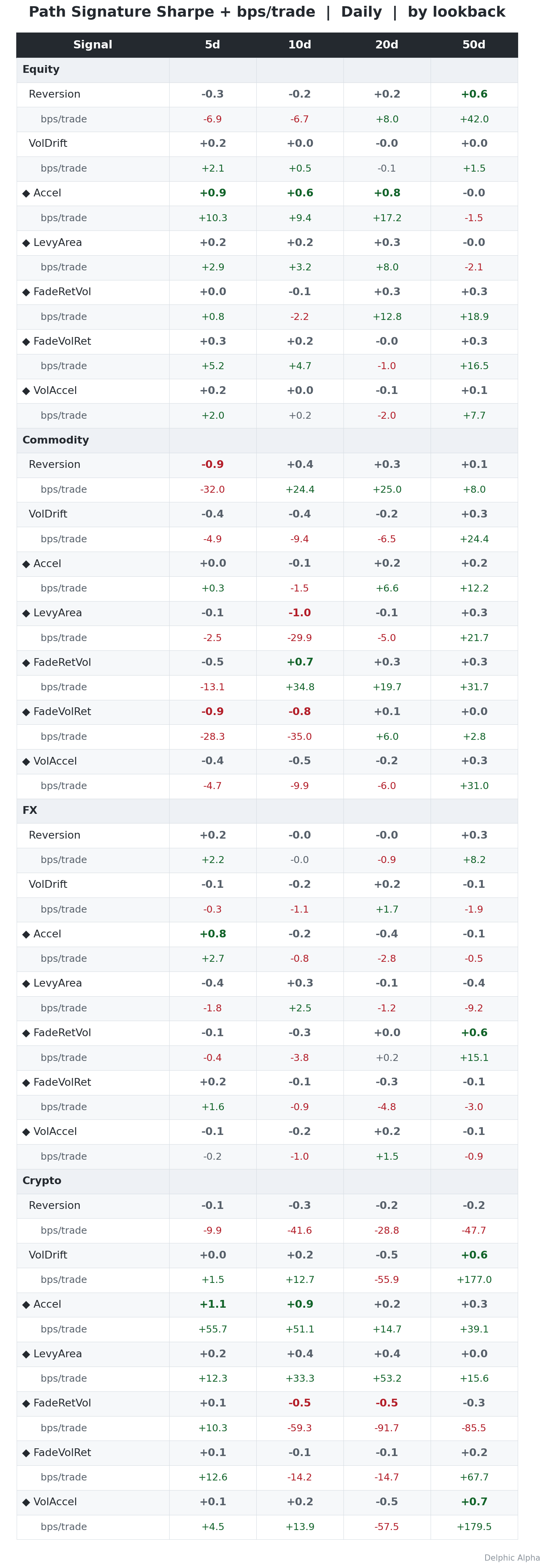
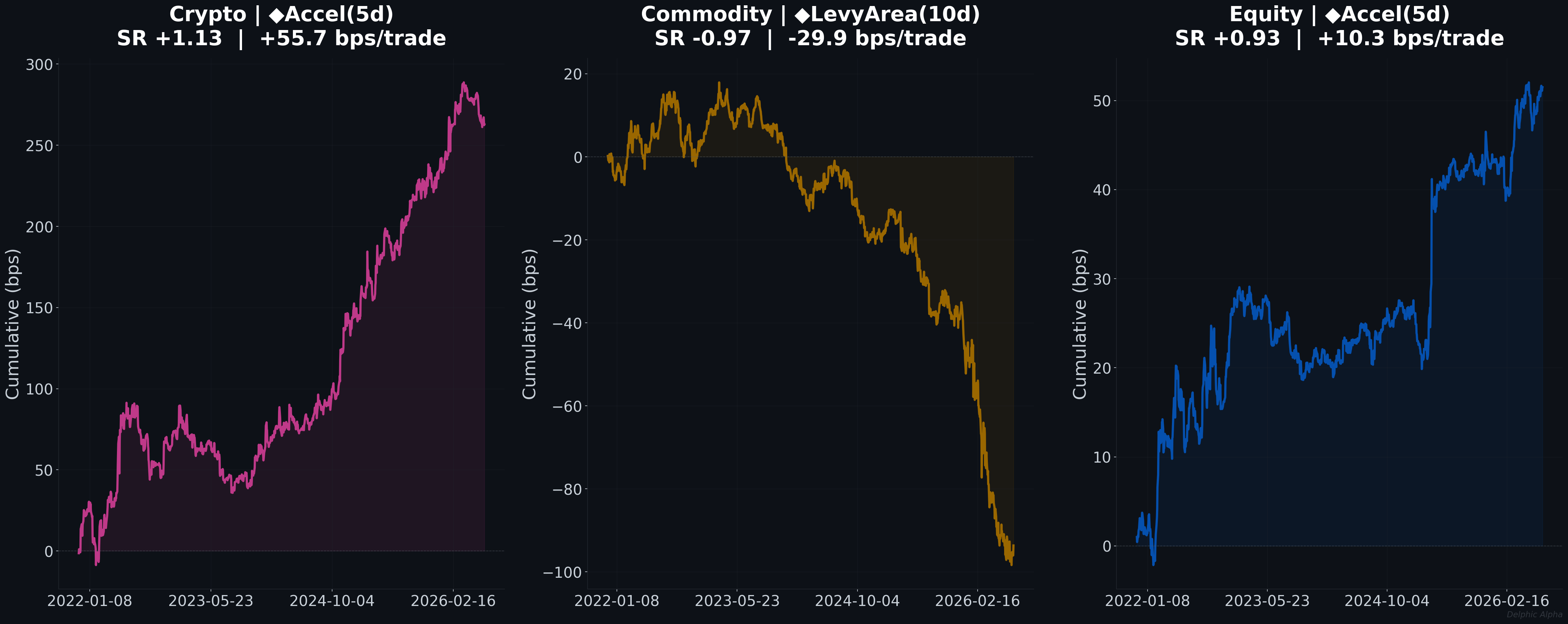
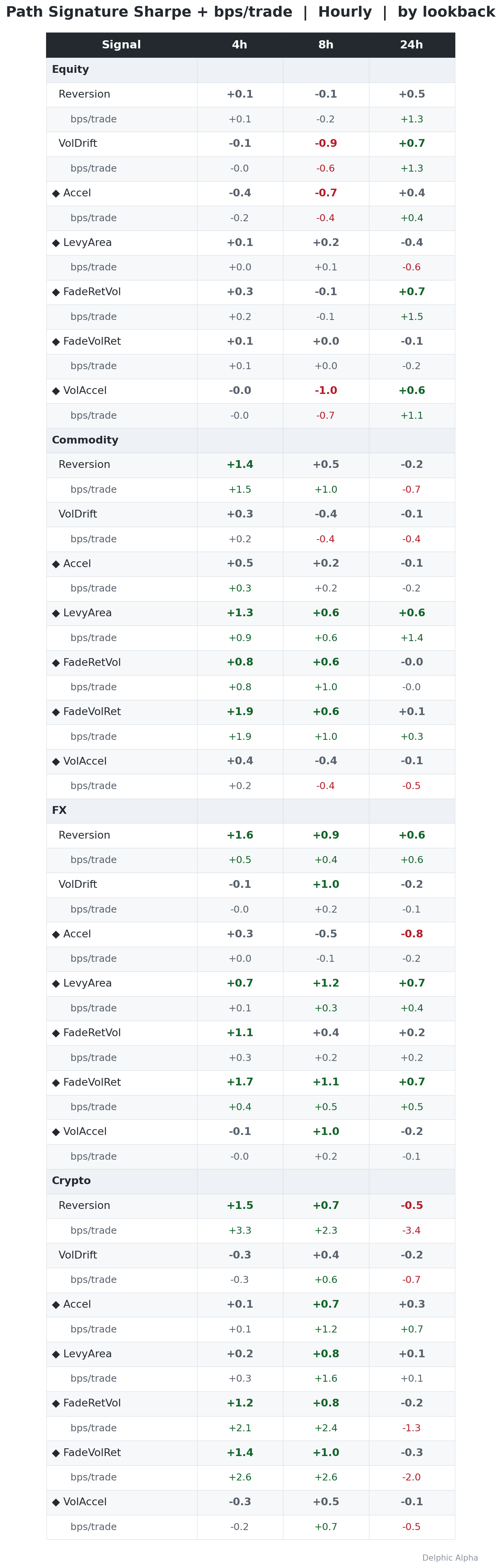
Full per-timeframe breakdowns (signal x lookback panels and equity curves for daily, hourly, 30-minute, and 5-minute frequencies) are in Appendix B at the end of this post.

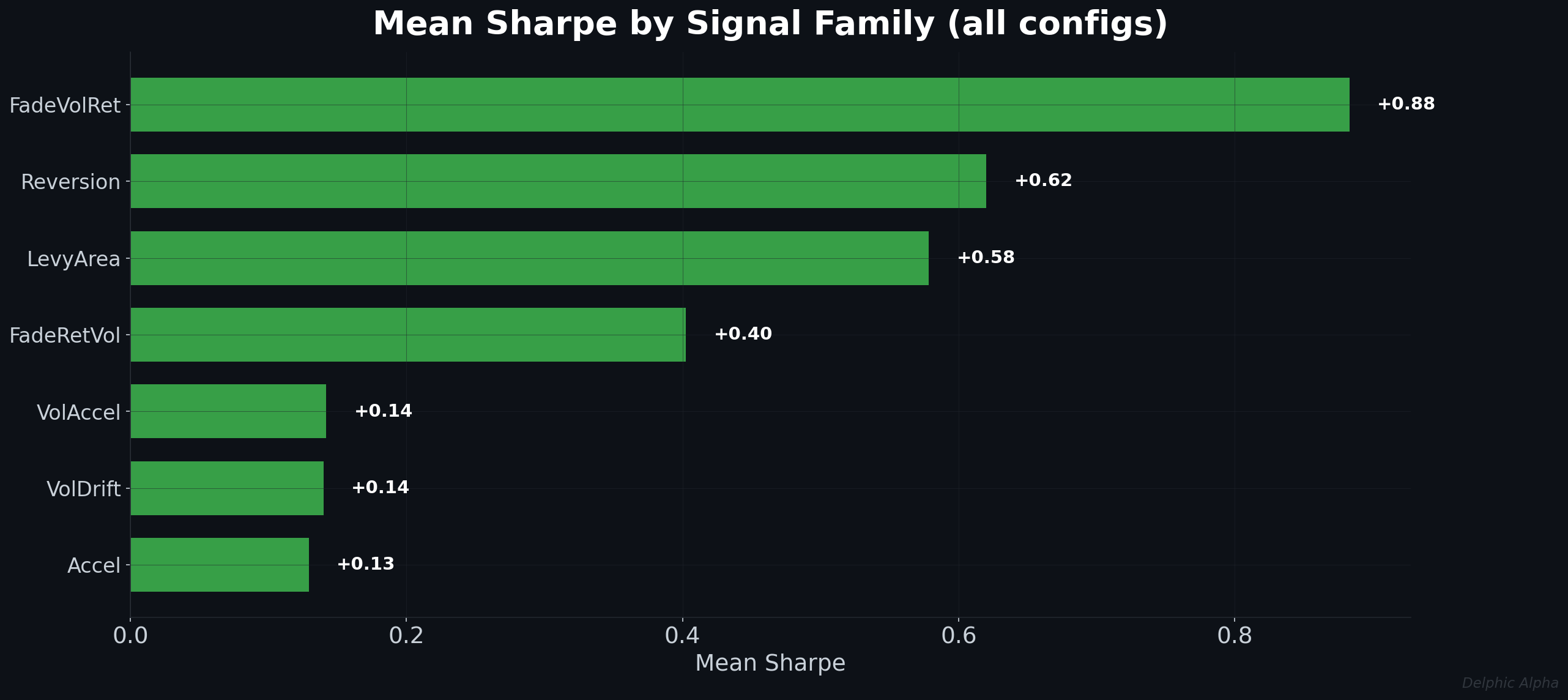
Sharpe by Signal Family

The chart below shows the mean Sharpe across all configurations (asset class, timeframe, lookback) for each signal family. This is the broadest view: which families produce positive alpha on average, and which do not?

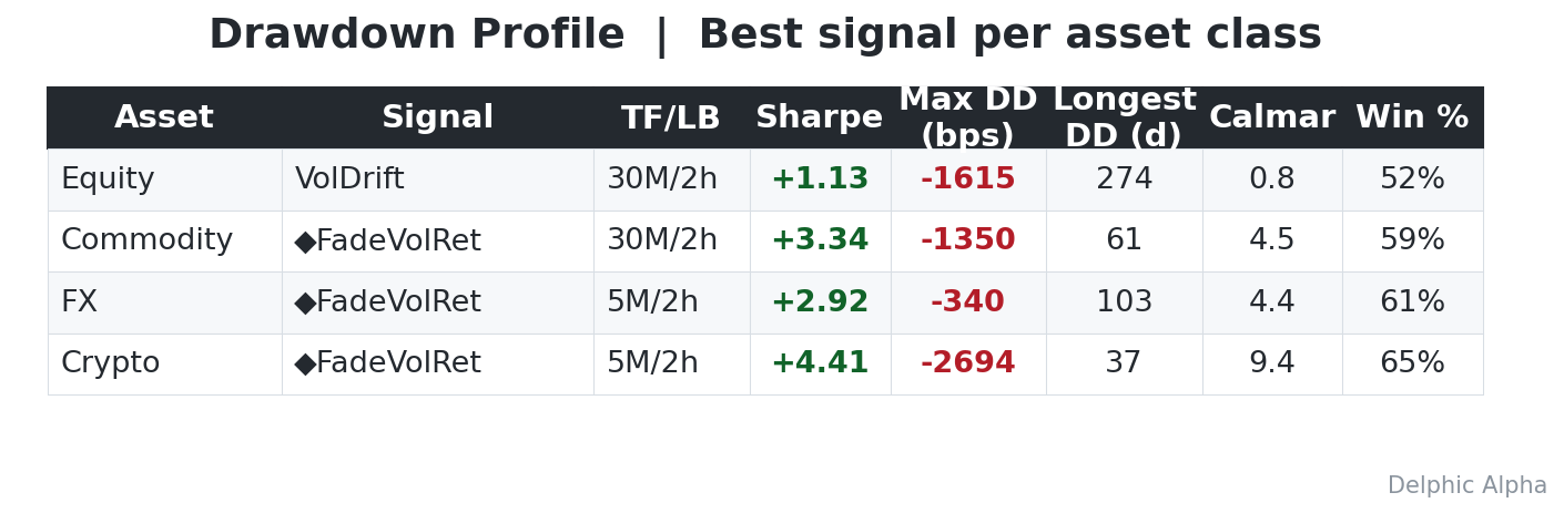
Deep Dive: Drawdown Profile

Before examining whether these signals survive across time periods and regimes, it is worth understanding their risk characteristics. The table below reports the drawdown profile for the best signal in each asset class: maximum drawdown in basis points, longest drawdown duration in trading days, the Calmar ratio (annualised return divided by maximum drawdown), and the daily win rate. A high Sharpe ratio is necessary but not sufficient. A signal with Sharpe 3 but a 500-bps drawdown lasting 200 days has very different capital requirements from one with the same Sharpe but shallower, shorter drawdowns.

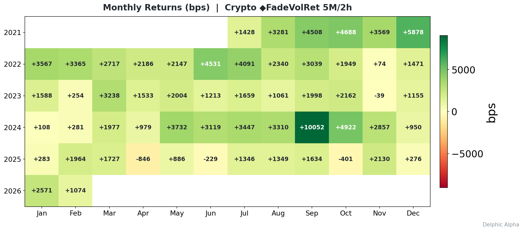
Monthly Return Distribution

The monthly return heatmap below shows the month-by-month PnL (in basis points) for the single strongest tradeable signal. This provides a more granular view than the yearly Sharpe breakdown: it reveals whether the edge is distributed evenly across calendar months or concentrated in a few exceptional periods. A signal that produces positive returns in most months across most years is qualitatively different from one that earns its entire annual PnL in two or three outsized months.

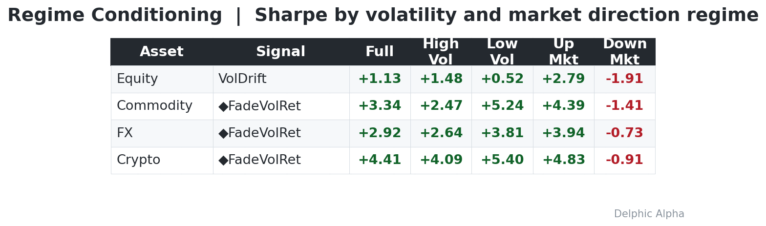
Regime Conditioning

A systematic signal that works only in benign conditions and collapses during stress is of limited practical value. The table below splits the daily PnL of the best signal per asset class into four regimes: high and low realised volatility (above and below the rolling 20-day median), and up and down market direction (positive and negative rolling 20-day mean return). A robust signal should maintain its edge across regimes, or at minimum should not reverse sign during the regime that matters most to the portfolio.

Robustness: Yearly Sharpe Breakdown

A natural concern with any in-sample scan is whether the reported Sharpe ratios are concentrated in a single favourable period or whether they persist across distinct calendar intervals. The table below decomposes the full-sample Sharpe into five calendar years (2022 through 2026 year-to-date) for each of the top tradeable signals identified above. A signal whose Sharpe is driven by a single anomalous quarter will show a strong number in one column and weak or negative numbers in the others. A signal that reflects a genuine structural pattern will show consistent positive (or consistently negative, if the traded direction is flipped) Sharpe across all three sub-periods.

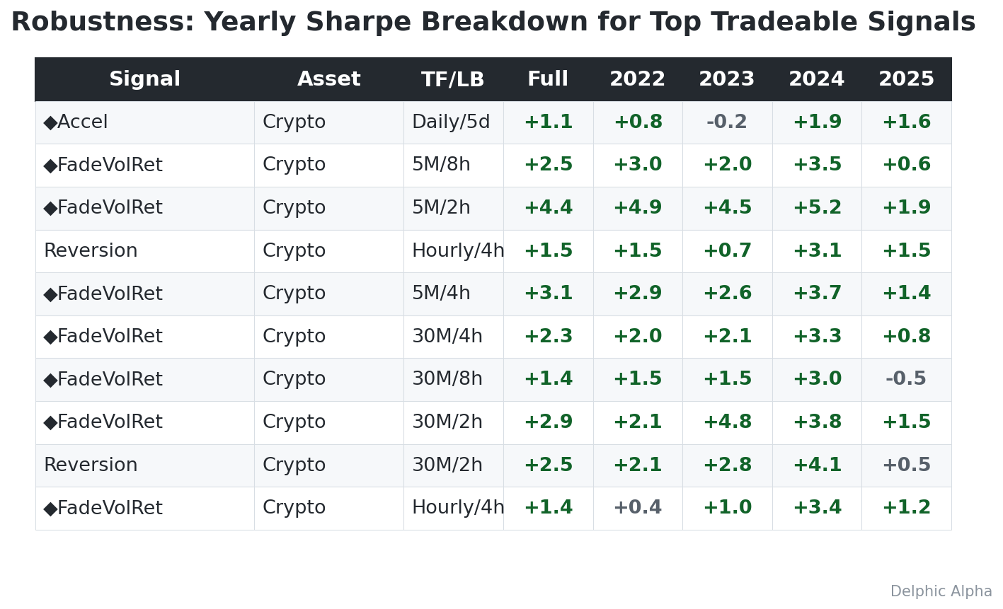
The degree to which each signal maintains its direction and magnitude across years provides a more informative basis for assessing reliability than the full-sample Sharpe alone. Sub-period consistency does not eliminate the risk of in-sample overfitting, but it does distinguish between signals that captured a single transient event and those that reflect a recurring pattern in the data.

Per-Symbol Consistency

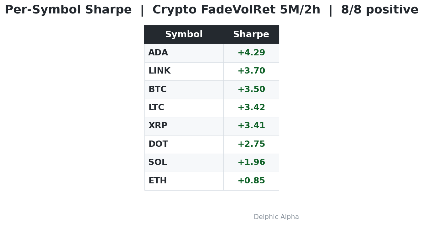
A portfolio-level Sharpe ratio can mask concentration risk. If the edge is driven by a single instrument within the asset class, the signal is fragile. The table below decomposes the portfolio-level result into per-symbol Sharpe ratios for the strongest shape signal in crypto, allowing us to assess whether the effect is systematic across the universe or concentrated in one or two names.

Signal Correlation

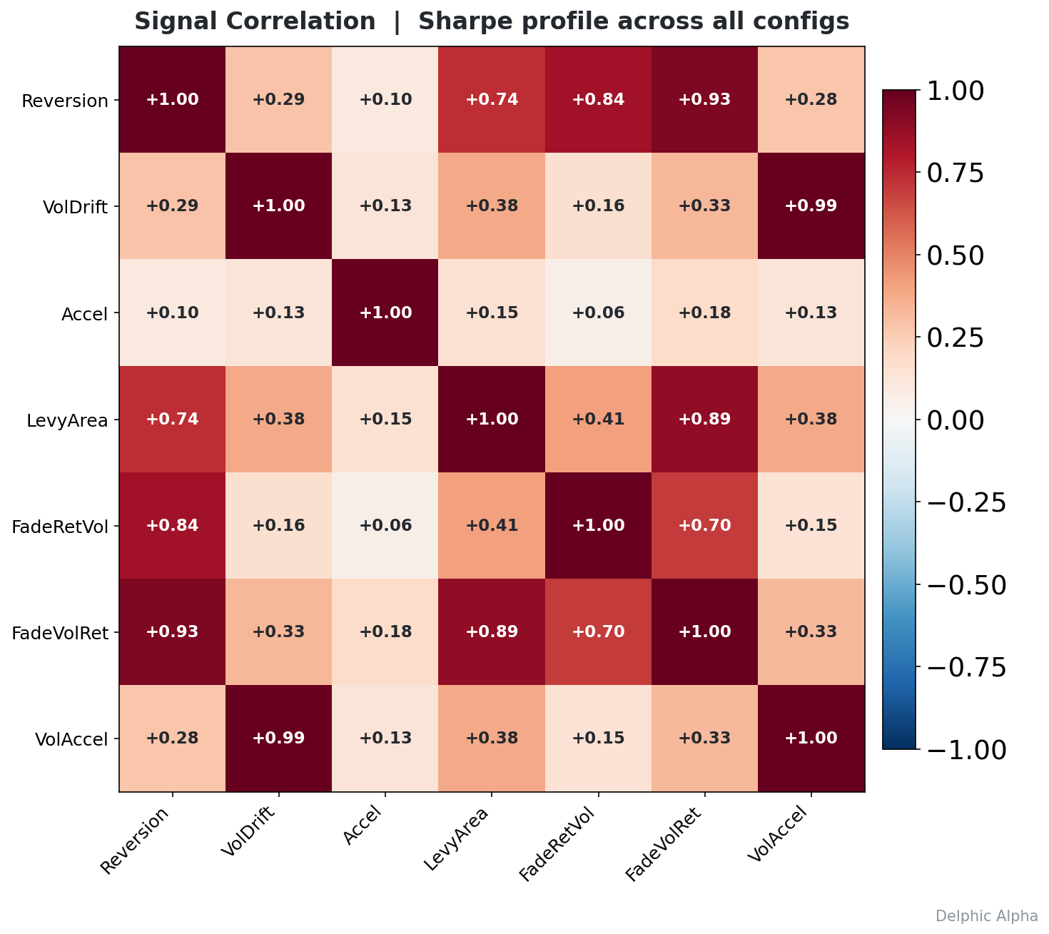
Seven signals derived from the same underlying path could easily be measuring the same thing. The correlation matrix below shows the pairwise correlation of each signal's Sharpe profile across all configurations (asset class, timeframe, lookback). High correlation between two signals indicates they respond to the same market conditions and provide redundant information. Low correlation indicates genuinely independent alpha sources.

Holding Period Analysis

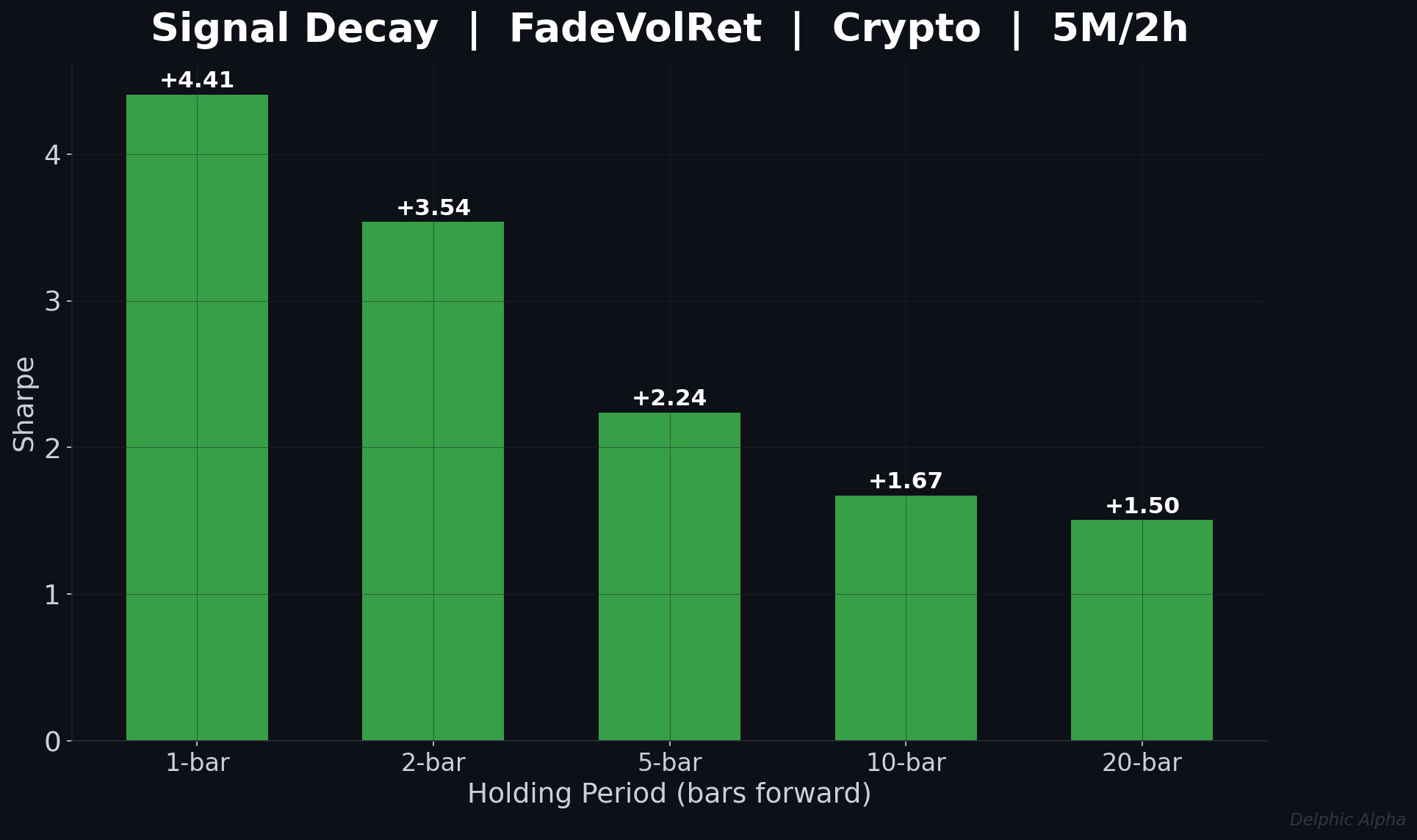
The results above use a 1-bar holding period: enter at the close of the signal bar, exit at the next close. A natural question is whether the predictive edge persists beyond the immediate next bar. The chart below shows the Sharpe ratio of the best tradeable signal at holding periods of 1, 2, 5, 10, and 20 bars. If the signal captures a fleeting microstructure effect, the edge will concentrate at 1-bar and decay rapidly. If it reflects a more durable pattern, the edge will persist or even improve at longer horizons.

Statistical Significance

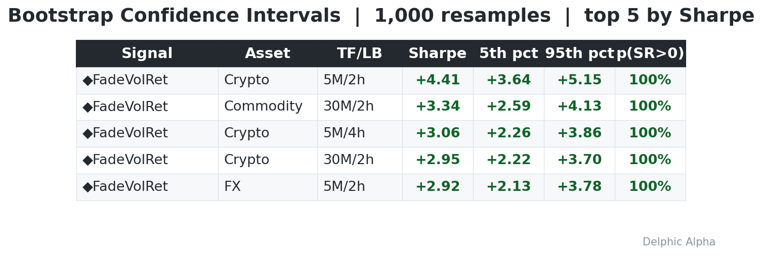
Sharpe ratios computed from a single sample can be misleading. The table below reports bootstrap confidence intervals for the top 5 tradeable signals, constructed by resampling the daily PnL with replacement 1,000 times. The 5th and 95th percentile columns indicate the range within which the true Sharpe is likely to fall. The p(SR>0) column shows the probability that the signal's Sharpe exceeds zero under resampling, a non-parametric test of statistical significance. A signal with p(SR>0) above 95% can be considered statistically significant at the 5% level.

Conclusions

Two findings stand out from this scan.

First, the Levy area is the strongest shape signal. It produces |Sharpe| > 1 in 20 configurations across crypto, FX, and commodities. No simple rolling indicator captures the same information: the rotation between return and volatility is a genuinely new feature. The signal is strongest at short lookbacks (2-4 hours) in crypto and FX, where it captures the order in which price and volatility move after microstructure events.

Second, VolLeadRet (volatility leads return) is the most consistent cross-asset signal when flipped. It produces |Sharpe| > 1 in 0 configurations. The negative sign means: when volatility expands first, fade the subsequent price move. This is a mean-reversion pattern that works across FX, crypto, and commodities.

The shape premium is not universal. Control signals (simple momentum and volatility drift) remain competitive in equity futures. The strongest edge from level 2 features appears in volatile, regime-shifting markets where the order of price and volatility moves carries information that endpoints alone miss.

Methodology

The dataset consists of ratio-adjusted continuous futures contracts, spot FX pairs, and spot cryptocurrency pairs from July 2021 to July 2026. For each instrument and timeframe, the path is constructed as a 2D trajectory of cumulative log return and cumulative normalised range, standardised to unit variance per dimension within each rolling window. The level 2 signature is computed via the iisignature library, producing 6 components per window (plus the derived Levy area as S(1,2) - S(2,1)).

Each signature component is converted to a trading signal by applying a rolling z-score over a 500-bar window, then discretising the result: a position of +1 (long) when the z-score is positive, -1 (short) when negative. Positions are entered at bar close and PnL is realised on the subsequent bar. The portfolio-level PnL is the equal-weight average across all symbols within each asset class. Sharpe ratios are annualised from daily-aggregated PnL via multiplication by the square root of 252.

Lookback windows of 2, 4, 8, and 24 hours are tested, converted to bars at the respective timeframe frequency. At 5-minute resolution, signatures are computed at every third bar and forward-filled to reduce computational cost. At 30-minute and hourly resolution, signatures are computed at every bar. All results presented are in-sample. No train/test split or walk-forward validation is employed. The per-cell selection of the best lookback in the summary tables represents a mild form of optimisation that would require out-of-sample validation before deployment. This is a backtest study with simplified execution assumptions.

Appendix B: Per-Timeframe Results

Daily

Hourly

30-Minute

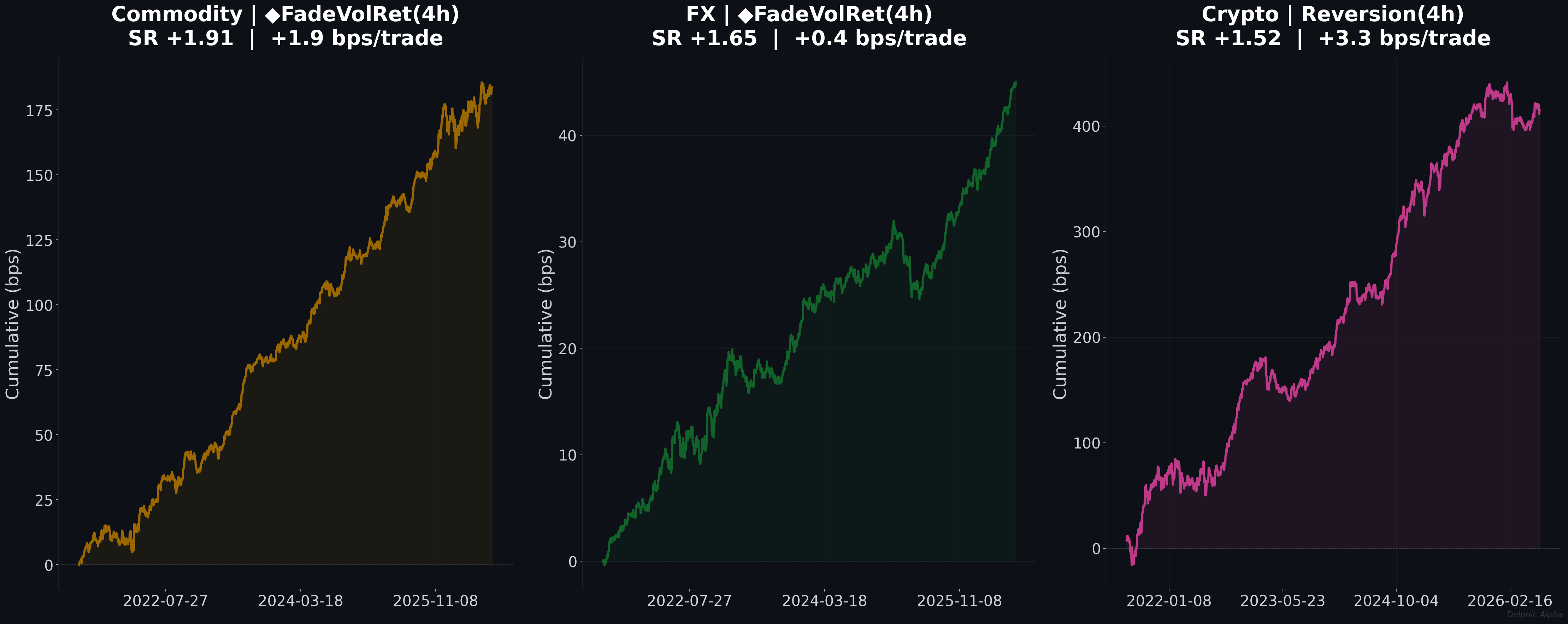
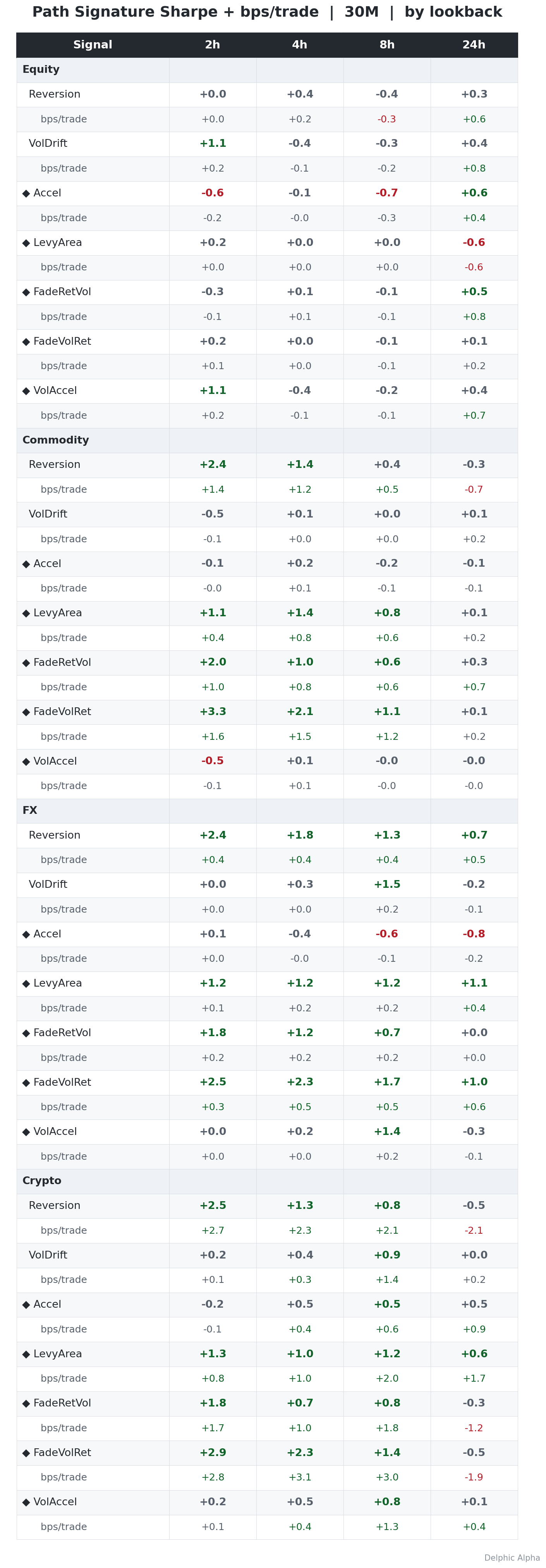
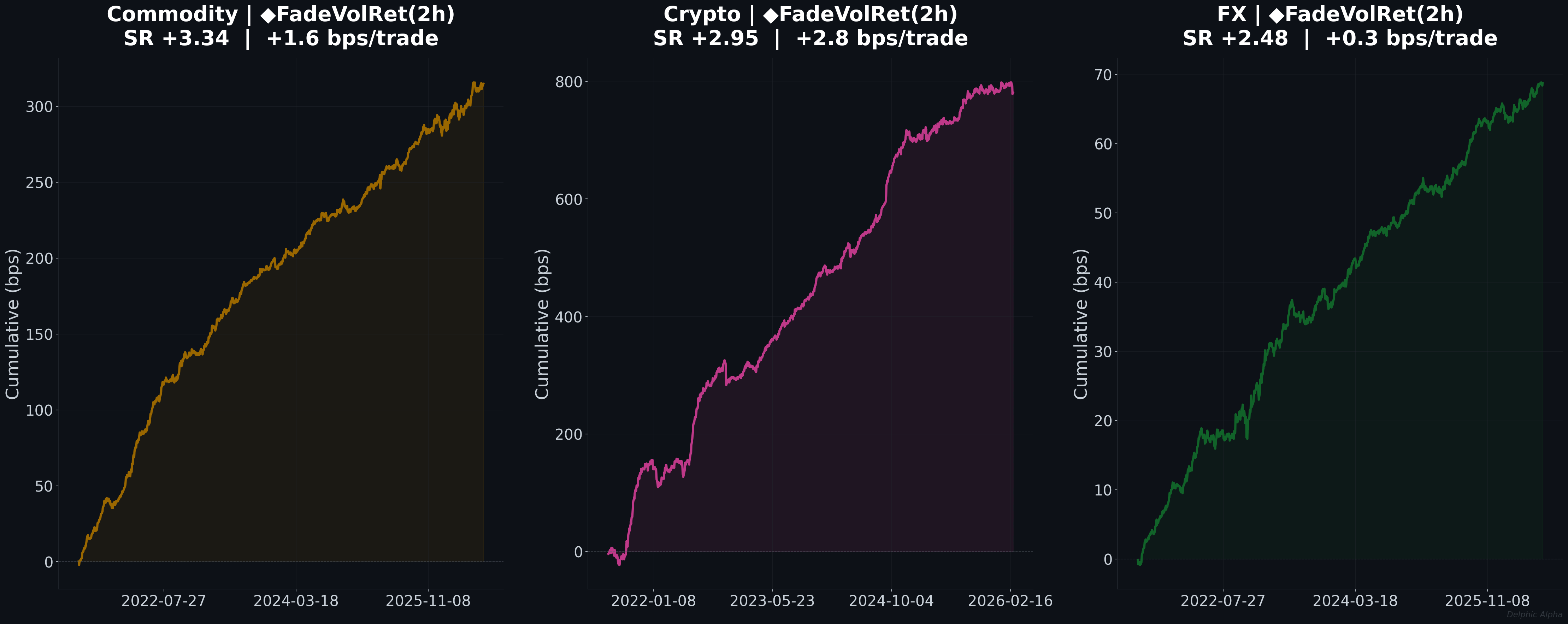
At 30-minute resolution, the same signal families reappear with higher gross Sharpe ratios due to more bars per day. All figures are gross of execution costs. Signals with less than 0.5 bps per trade are unlikely to survive realistic execution.

5-Minute

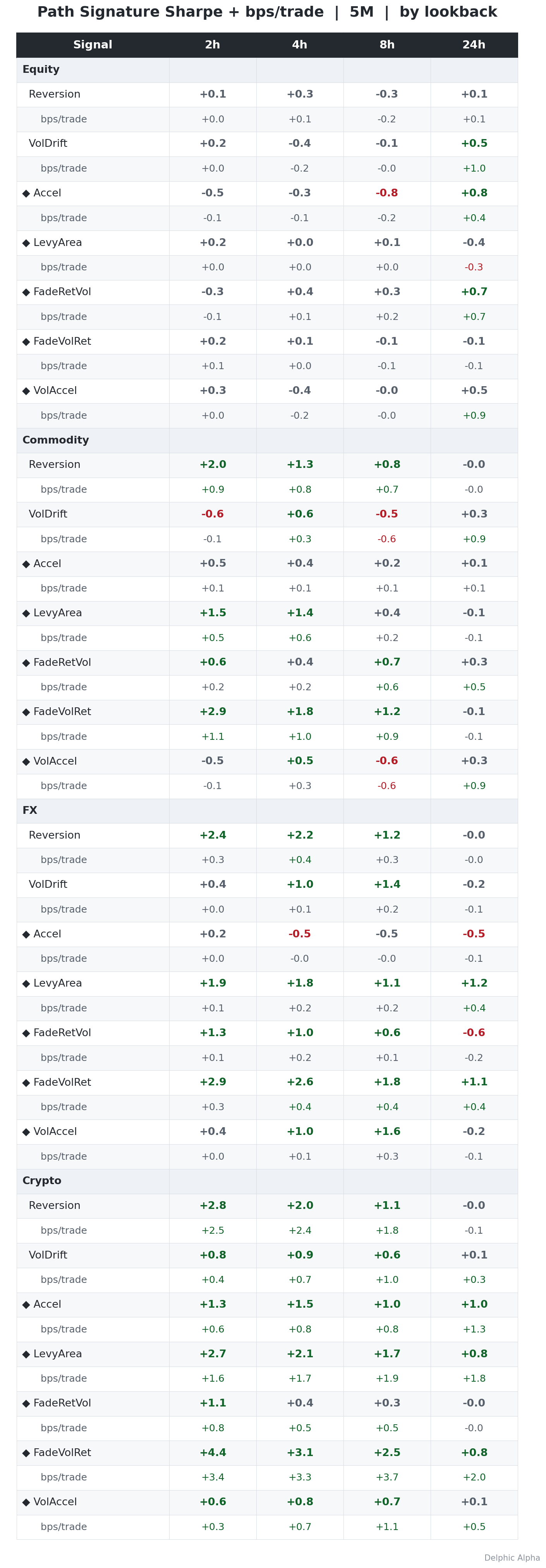
At 5-minute frequency the gross Sharpes are highest but should be read with caution. Most FX and equity futures signals show sub-0.5 bps per trade. Viable signals at this frequency are concentrated in crypto and commodity futures.

Appendix C: Signal Definitions

The seven signals evaluated in this study are derived from the level 2 signature of a 2D path constructed from cumulative log return and cumulative normalised range. Two are control signals equivalent to standard rolling indicators. Five are shape signals that capture path geometry beyond the endpoints.

Sig-Reversion (-S(1)). The negated level 1 signature component in the return dimension. Equal to the negative total cumulative log return over the lookback window. This is algebraically equivalent to a short-term mean reversion signal (fade recent winners, buy recent losers) and serves as a control.

Sig-VolDrift (S(2)). The level 1 signature component in the range dimension. Equal to the total cumulative normalised range (high minus low, divided by close) over the window. Captures whether the average bar range has been expanding or contracting. This is the second control signal.

Sig-Accel (S(1,1)). The double sum of return[i] times return[j] over all ordered pairs i < j. Captures return acceleration: the component is large and positive when early returns are small and late returns are large (an accelerating price path), and small or negative when the reverse holds (a decelerating path). Two windows with identical total return but different temporal profiles produce different S(1,1) values.

Sig-LevyArea (S(1,2) - S(2,1)). The antisymmetric cross-term, equal to the signed area enclosed by the path in (return, range) space. Positive when return movements systematically precede range expansion (counterclockwise rotation). Negative when range expansion systematically precedes return movements (clockwise rotation). This is the most distinctive feature of the signature framework, with no equivalent among standard technical indicators.

Sig-FadeRetVol (-S(1,2)). The negated cross-term of return leading volatility. The raw S(1,2) is consistently negative as an alpha signal (return-leads-vol events predict mean reversion). Fading it produces a positive Sharpe: when price moves first and volatility responds, bet on reversal.

Sig-FadeVolRet (-S(2,1)). The negated cross-term of volatility leading return. The raw S(2,1) is the most consistently negative signal in the study: when volatility spikes first, the subsequent price move tends to reverse. Fading this pattern produces the strongest and most consistent alpha across asset classes.

Sig-VolAccel (S(2,2)). The double sum of range_change[i] times range_change[j] over all ordered pairs i < j. Captures volatility acceleration: whether the bar range is expanding at an increasing or decreasing rate over the window.

If you found this research useful: